Equilibrium Solutions Of Differential Equations

Bear witness Mobile Notice Show All NotesHibernate All Notes

Mobile Notice

You appear to be on a device with a "narrow" screen width (i.east. you are probably on a mobile phone). Due to the nature of the mathematics on this site information technology is all-time views in mural mode. If your device is not in mural mode many of the equations volition run off the side of your device (should be able to scroll to run across them) and some of the carte du jour items volition exist cut off due to the narrow screen width.

Department 2-8 : Equilibrium Solutions

In the previous section we modeled a population based on the assumption that the growth rate would be a abiding. Still, in reality this doesn't make much sense. Clearly a population cannot be allowed to abound forever at the same charge per unit. The growth charge per unit of a population needs to depend on the population itself. Once a population reaches a certain betoken the growth rate volition first reduce, frequently drastically. A much more than realistic model of a population growth is given past the logistic growth equation. Here is the logistic growth equation.

\[P' = r\left( {one - \frac{P}{1000}} \correct)P\]

In the logistic growth equation $r$ is the intrinsic growth charge per unit and is the same $r$ every bit in the last section. In other words, it is the growth rate that will occur in the absence of whatever limiting factors. $Yard$ is chosen either the saturation level or the carrying capacity.

Now, nosotros claimed that this was a more than realistic model for a population. Allow's see if that in fact is correct. To allow united states to sketch a management field permit'south pick a couple of numbers for $r$ and $Thou$. We'll utilize $r = \frac{i}{2}$ and $M = x$. For these values the logistics equation is.

\[P' = \frac{one}{2}\left( {1 - \frac{P}{{10}}} \correct)P\]

If you lot need a refresher on sketching management fields go dorsum and take a await at that department. First notice that the derivative will be zero at $P = 0$ and $P = 10$. Also notice that these are in fact solutions to the differential equation. These ii values are called equilibrium solutions since they are constant solutions to the differential equation. We'll leave the rest of the details on sketching the direction field to you. Here is the direction field as well every bit a couple of solutions sketched in besides.

$A graph with domain $0 \le t \le 8$ and range $0 \le P(t) \le 14$. At P(t)=x and P(t)=0 there are horizontal lines of arrows all pointing to the correct. Below P(t)=0 there are arrows with a decreasing slope. In the range 0< P(t)<x there are a series of increasing arrows. Arrows that start well-nigh P(t)=0 all have a shallow and increasing slope. Every bit you move away from P(t)=0 the arrows steepen out and and then every bit they almost P(t)=10 they start to shallow back out. To a higher place P(t)=10 there are a series of decreasing arrows. Arrows that are near P(t)=50 all accept a shallow and decreasing gradient. The further to a higher place P(t)=10 the arrows go the steeper (and still decreasing) their slopes are. Forth the P(t) axis a number of graph representing solutions start. All of the graphs are parallel to the arrows. The graphs at P(t) = 0 and P(t)=10 are a horizontal lines. Solutions that start above P(t)=10 all decrease towards P=x and shallow out as they get closer to P=ten without really crossing. Solutions in the range 0<P<10 all increase until they get close to P=10 and then shallow out as they get closer to P=10 without actually crossing.$

Note, that we included a small portion of negative $P$'s in here fifty-fifty though they really don't make whatsoever sense for a population trouble. The reason for this volition be credible downwards the road. Likewise, notice that a population of say 8 doesn't make all that much sense then let's assume that population is in thousands or millions so that viii actually represents eight,000 or eight,000,000 individuals in a population.

Observe that if nosotros outset with a population of zero, there is no growth and the population stays at goose egg. Then, the logistic equation volition correctly effigy out that. Side by side, observe that if we first with a population in the range $0 < P\left( 0 \right) < ten$ then the population volition grow, but beginning to level off once we become shut to a population of 10. If we start with a population of 10, the population will stay at 10. Finally, if we start with a population that is greater than 10, then the population will actually dice off until we start nearing a population of x, at which point the population decline volition start to slow down.

Now, from a realistic standpoint this should make some sense. Populations can't just abound forever without bound. Somewhen the population will reach such a size that the resources of an surface area are no longer able to sustain the population and the population growth will start to irksome as information technology comes closer to this threshold. Also, if you start off with a population greater than what an surface area tin can sustain there volition really exist a die off until we get well-nigh to this threshold.

In this example that threshold appears to be 10, which is also the value of $K$ for our trouble. That should explain the proper noun that we gave $K$ initially. The carrying capacity or saturation level of an surface area is the maximum sustainable population for that expanse.

So, the logistics equation, while nevertheless quite simplistic, does a much improve job of modeling what will happen to a population.

Now, permit's move on to the point of this section. The logistics equation is an instance of an democratic differential equation. Autonomous differential equations are differential equations that are of the form.

\[\frac{{dy}}{{dt}} = f\left( y \right)\]

The but place that the contained variable, $t$ in this case, appears is in the derivative.

Notice that if $f\left( {{y_0}} \correct) = 0$ for some value $y = {y_0}$ and then this will also be a solution to the differential equation. These values are called equilibrium solutions or equilibrium points. What we would similar to do is classify these solutions. By classify we mean the post-obit. If solutions outset "almost" an equilibrium solution will they move abroad from the equilibrium solution or towards the equilibrium solution? Upon classifying the equilibrium solutions we tin can then know what all the other solutions to the differential equation will do in the long term simply past looking at which equilibrium solutions they starting time near.

So, just what do nosotros mean past "nigh"? Go dorsum to our logistics equation.

\[P' = \frac{1}{two}\left( {1 - \frac{P}{{10}}} \right)P\]

As nosotros pointed out at that place are two equilibrium solutions to this equation $P = 0$ and $P = x$. If we ignore the fact that we're dealing with population these points break upward the $P$ number line into three distinct regions.

\[ - \infty < P < 0\hspace{0.25in}\hspace{0.25in}\hspace{0.25in}\,\,\,\,0 < P < ten\hspace{0.25in}\hspace{0.25in}\hspace{0.25in}\,x < P < \infty \]

We will say that a solution starts "near" an equilibrium solution if information technology starts in a region that is on either side of that equilibrium solution. Then, solutions that outset "near" the equilibrium solution $P = x$ will commencement in either

\[0 < P < ten\hspace{0.25in}{\mbox{OR}}\hspace{0.25in}\,10 < P < \infty \]

and solutions that get-go "virtually" $P = 0$ will start in either

\[ - \infty < P < 0\hspace{0.25in}\,\,\,{\mbox{OR}}\hspace{0.25in}\,\,\,\,\,\,0 < P < 10\]

For regions that lie between two equilibrium solutions we tin can think of any solutions starting in that region as starting "nigh" either of the two equilibrium solutions equally we need to.

Now, solutions that start "near" $P = 0$ all move away from the solution as $t$ increases. Note that moving away does not necessarily mean that they abound without bound as they move abroad. Information technology but means that they motility away. Solutions that commencement out greater than $P = 0$ move away but do stay bounded as $t$ grows. In fact, they move in towards $P = x$.

Equilibrium solutions in which solutions that start "near" them motion abroad from the equilibrium solution are called unstable equilibrium points or unstable equilibrium solutions. So, for our logistics equation, $P = 0$ is an unstable equilibrium solution.

Next, solutions that start "near" $P = x$ all move in toward $P = 10$ every bit $t$ increases. Equilibrium solutions in which solutions that starting time "about" them move toward the equilibrium solution are called asymptotically stable equilibrium points or asymptotically stable equilibrium solutions. And so, $P = 10$ is an asymptotically stable equilibrium solution.

At that place is ane more than classification, but I'll wait until we become an example in which this occurs to innovate it. So, let's take a wait at a couple of examples.

Case one Notice and classify all the equilibrium solutions to the following differential equation.

\[y' = {y^2} - y - six\]

Evidence Solution

Commencement, find the equilibrium solutions. This is generally easy enough to practice.

\[{y^2} - y - 6 = \left( {y - 3} \right)\left( {y + 2} \right) = 0\]

So, it looks like we've got two equilibrium solutions. Both $y = -two$ and $y = 3$ are equilibrium solutions. Beneath is the sketch of some integral curves for this differential equation. A sketch of the integral curves or direction fields can simplify the process of classifying the equilibrium solutions.

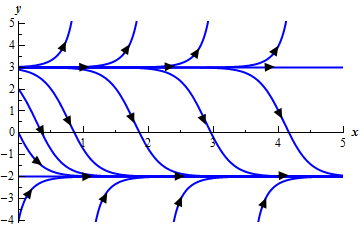
$A graph with domain $0 \le x \le 5$ and range $-5 \le y \le 5$. There are a series of sketches of solutions on the graph. At y=-2 and y=3 the solutions are horizontal lines. Solutions that first beneath y=-2 all increase up towards y=-ii shallowing out every bit they become near y=-2 without actually crossing. Graphs in the range -2<y<3 start near y=3 and are shallow decreasing graphs. As they move down from y=3 they steepen out and the start to shallow back out as they get near y=-2 without actually crossing. Graphs starting above y=3 all increase away from y=3.$

From this sketch information technology appears that solutions that start "virtually" $y = -2$ all motility towards it equally $t$ increases and then $y = -two$ is an asymptotically stable equilibrium solution and solutions that commencement "near" $y = 3$ all move away from information technology equally $t$ increases and and then $y = three$ is an unstable equilibrium solution.

This next case volition introduce the tertiary classification that we tin give to equilibrium solutions.

Example 2 Discover and allocate the equilibrium solutions of the following differential equation.

\[y' = \left( {{y^2} - iv} \right){\left( {y + 1} \right)^2}\]

Show Solution

The equilibrium solutions are to this differential equation are $y = -2$, $y = 2$, and $y = -1$. Below is the sketch of the integral curves.

$A graph with domain $0 \le x \le 5$ and range $-3 \le y \le 3$. There are a series of sketches of solutions on the graph. At y=-2, y=-1 and y=2 the solutions are horizontal lines. Solutions that start below y=-two all increase up towards y=-two shallowing out as they get well-nigh y=-ii without actually crossing. Graphs in the range -2<y<-1 start near y=-1 and are shallow decreasing graphs. As they move down from y=-1 they steepen out and the outset to shallow dorsum out equally they become about y=-2 without actually crossing. Graphs in the range -ane<y<2 start near y=2 and are shallow decreasing graphs. As they move down from y=2 they steepen out and the start to shallow back out as they get near y=-1 without actually crossing. Graphs starting above y=2 all increase away from y=2.$

From this information technology is clear (hopefully) that $y = 2$ is an unstable equilibrium solution and $y = -2$ is an asymptotically stable equilibrium solution. Even so, $y = -i$ behaves differently from either of these two. Solutions that start above it move towards $y = -one$ while solutions that start below $y = -1$ motility away every bit $t$ increases.

In cases where solutions on one side of an equilibrium solution move towards the equilibrium solution and on the other side of the equilibrium solution move away from information technology we call the equilibrium solution semi-stable.

So, $y = -i$ is a semi-stable equilibrium solution.